Working with SQL Window Functions

SQL Window FunctionsSQL Window Functions

DuckDB provides 14 SQL window-related functions in addition to all the aggregation functions that can be combined with windows. Snowflake, on the other hand, offers more than 70 functions that can be used with SQL windows. PostgreSQL also supports 11 SQL window-related functions, as well as all the aggregation functions that are packaged by default, in addition to any user-provided aggregation function.

Hopefully, the above information has captured your attention and helped you realize how important SQL windows are, based on the effort database vendors are making to add support for them.

But what’s a window in SQL?

The concept of windows is actually pretty simple. It allows us to perform calculations across sets of rows that are related to the current row in some way.

Think of iterating through all the rows but the calculation we want to perform is related not just to the current row values but also to a subset of the total rows.

Another way to think about window functions is by considering the GROUP BY semantics. When we use GROUP BY we are asking SQL to compute a function by grouping first the data using the parameters of the GROUP BY clause. Consider the following SQL

 select user_id, count(events) as total_actions from user_activity group by user_id;

In the above example, we ask SQL to split events among unique user_ids and count them for each user separately. Both the calculation but also the grouping results will be included at the resulting table. So for example:

user_id	event
1	click
2	click
2	load
1	load
1	load

Assuming the above input table, the result of the query will look like this:

user_id	total_actions
1	3
2	2

You can think of SQL Windows as something similar in how data is processed but without having necessarily to present the results grouped at the end.

But windows are actually even more powerful as we will see.

What comes after partitioning ?

As we’ve seen previously, partitioning is a first important concept to understand about windows. We can create sub-sets from our data and perform calculations only inside these sub-sets and the main mechanism for defining the sets, is by describing to SQL how to partition the data.

But we can do more than that! See the example below,

Here’s an example SQL query that uses a window function and the LAG() function to calculate the time lapse between consecutive events:

SELECT
  event_time,
  event_type,
  user_id,
  event_time - LAG(event_time) OVER (PARTITION BY user_id ORDER BY event_time) AS time_lapse
FROM
  user_activity

This query partitions the data by user_id and orders it by event_time. Remember what we said previously about partitioning? You see it here in action. We want our calculation to be performed for each user we have so we will partition on it.

We will also sort our data based on event_time, the reason we do that, is because we want to calculate the time it took our user to perform one event after the other. The reason we are sorting is because of what we’ll do next.

Our query then uses theLAG() function, which is the window function that will do the magic for us. What LAG() does, is to make available the previous value to the current row we currently process, within our window!

The code part:

event_time - LAG(event_time)

Does exactly that, while we go through the current row’s event_time, we get access to the event_time value from the previous row and because the rows are sorted, we can now subtract the values and calculate the time lapse!

The window magic is defined in this part of the syntax:

event_time - LAG(event_time) OVER (PARTITION BY user_id ORDER BY event_time)

The OVERterm indicates the start of the window definition, just try to read this as a sentence written in english and it almost explains what is happening. That’s part of the beauty of being a declarative langue!

The difference is going to be calculated over sets of data that are created using the user_id, so we get one set of rows for each user and we also sort this set based on the event_time. What is important to remember here is that sorting is not global, instead data is sorted only assuming each individual set defined by the user_id.

After the partitions have been created and sorted, the query engine starts iterating the rows of each partition and at each one the LAG function will make the value of the previous row available to the engine.

At this point, everything is available for the engine to calculate the difference between the two values and that’s exactly what it does!

LAG() and the above example is a great introduction to the last important concept about windows in SQL. Framing!

Windows and Frames

Windowing breaks up a relation into independent groups or “partitions,” then orders those partitions and computes a new column for each row based on nearby values.

In many cases, the functions that we apply depend only on the partition boundary and maybe also the ordering, see the very simple first example we went through.

In other cases though, the function might need access to some of the previous or following values. This was the case with LAG in our previous example.

Although we had defined a partition based on the user_id, we also needed to provide to our function (in this case subtraction) with the previous to the current value. This is exactly what LAG did.

Frames are a generalization of this concept.

In our previous example, the frame was one row preceding our current row. Although we didn’t provide how many preceding rows we’d like to consider and thus LAG used the default which is 1 but we can use any number we want.

In DuckDB the definition of LAG is:

lag(expr any [, offset integer [, default any ]])

Offset refers to the number of rows preceding the current one that we want to access. We can also, set a default value to return if the requested offset does not exist. For example, if we are at the first row and want to access the previous one, we can define a default value to return instead.

Let’s consider the following table:

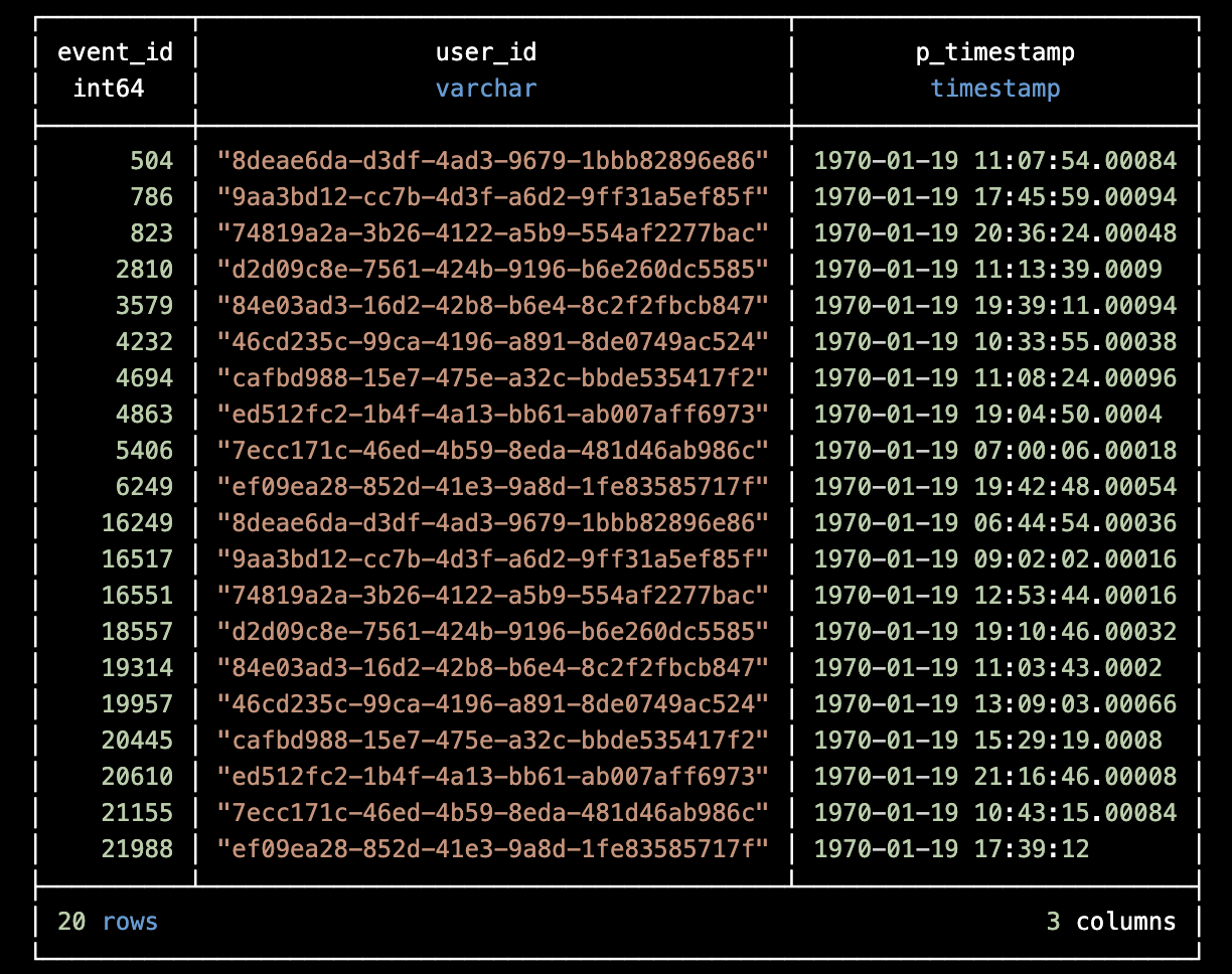To better understand the concepts of partitions versus frames, let’s see how the table will look like if we apply a window like the following:

p_timestamp - LAG(p_timestamp) OVER (PARTITION BY user_id ORDER BY p_timestamp)

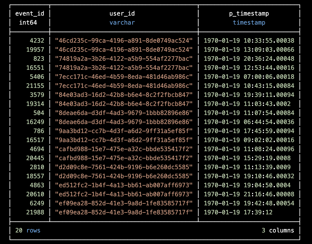
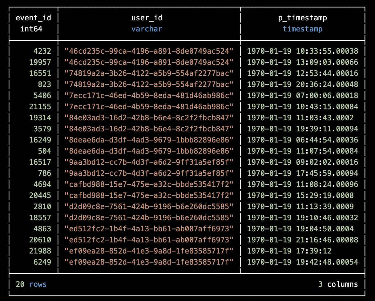
In the table below you can see how it will look like after the application of PARTITION BY. And this is how the table looks like after we order it. If you notice you will see that ordering exists only inside each partition and it’s not global.

You can think of the frame as a “window” sliding over the partitioned and ordered data, with a size equal to the offset parameter, in this case the offset is 1.

Consider that we are currently at row with event_id = 16249. The Frame will include this row and the previous one based on what we’ve said so far. What do you think the result of the Lag function will be from this frame?

The answer is 0. Remember that the frame has a default value equal to 0 which is returned when there’s no preceding row? Remember also that the frame has meaning only inside the boundaries of the partition?

The frame in this case is at the first position of the current partition and as a result the default value will be returned.

What about Nulls? Do they matter?

Null values always matter! 😀

We always should be aware of the null semantics around our window functions. Always check the documentation and see how the window function we care about is behaving in the presence of nulls.

For example in DuckDB, some functions can be configured to ignore nulls although the default behavior for all window functions is to respect them. Such an example is the LAG function that we used earlier.

In any case, make sure you understand well the semantics of your functions and the data you are working with. What if an aggregation function does a division by a null value?

Enough with theory, let’s have fun!

Ok, let’s work on some examples using window functions. For these examples we will be using DuckDB.

First, download DuckDB if you haven’t already. I’d recommend to just download the CLI but feel free to use any other way of working with DuckDB.

We will be working with JSON files so you will also need to install the JSON extension for DuckDB. To do that, you just have to:

#./duckdb

Enter ".help" for usage hints.
Connected to a transient in-memory database.
Use ".open FILENAME" to reopen on a persistent database.
D install 'json';

That’s all, now you are ready to start playing around and being dangerous.

The case of Sessionization

We will use a very common problem that requires window functions. We want to be pragmatic here, so using a real life example that you most probably will face sooner or later is what we are aiming for.

What is sessionization?

Assuming we have a number of user interactions captured in different moments in time, how can we group them into “meaningful” buckets. By meaningful in our context, we mean events that happened during one online session of the user.

The definition can get more complicated but this will suffice for our needs and to be honest it’s one of the most commonly used ones. For example, Google Analytics is using it as the default session definition.

The data

Now that we have the tools and the problem, we just need data and we are ready to go.

Again, we will try to be as realistic as possible. We will be using customer event data captured in the format supported by RudderStack and Segment.

These are the two most commonly used tools for capturing user interactions.

For more information on the whole schema of this format, you should check the amazing documentation provided here.

We will be using data that has been artificially generated, in case you’d like to generate your own data, you can use the tool I used. You can find it here.

I’ll also include a sample file that you can use directly! Using the event generator is useful if you want to experiment with different number of users and events and work on performance of your queries.

The queries

The first thing we have to do is to load our data into DuckDB and see how they look like.

Here I’ll assume that the file is named test.json and that it’s in the same path that you run duckdb from. Feel free to play around with paths etc, it helps to get a better grasp of how the CLI works and the SQL syntax of DuckDB.

D select * from read_json_objects('test.json') limit 2;

And if we execute the above, we’ll see something like this as output:

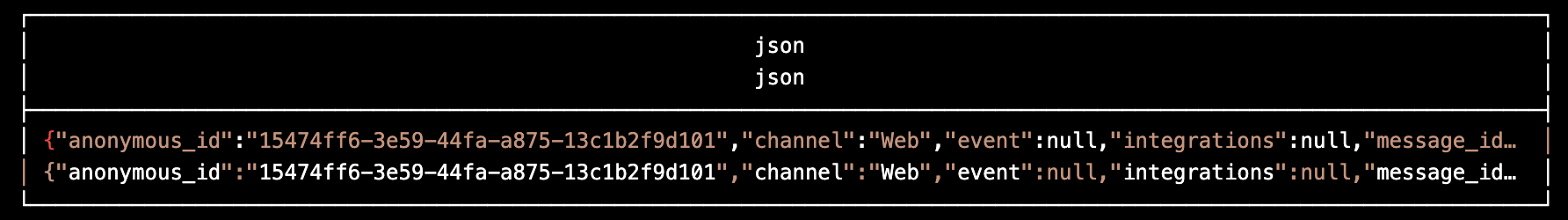
Although this worked, it’s not exactly useful yet. We just ended up with a table that has just one column of type json containing our json objects, one line of the input file corresponding to one row of the output table.

To make this more useful, we need to use some of the additional DuckDB magic for working with JSON.

consider the following query:

D select json_extract(json, '$.context.traits.id') as user_id,
		json_extract(json, '$.message_id') as event_id, 
		json_extract(json, '$.event_type') as event_type, 
		json_extract(json, 'original_timestamp') as original_timestamp 
	from js 
	limit 1;

The result you get should like something like this:

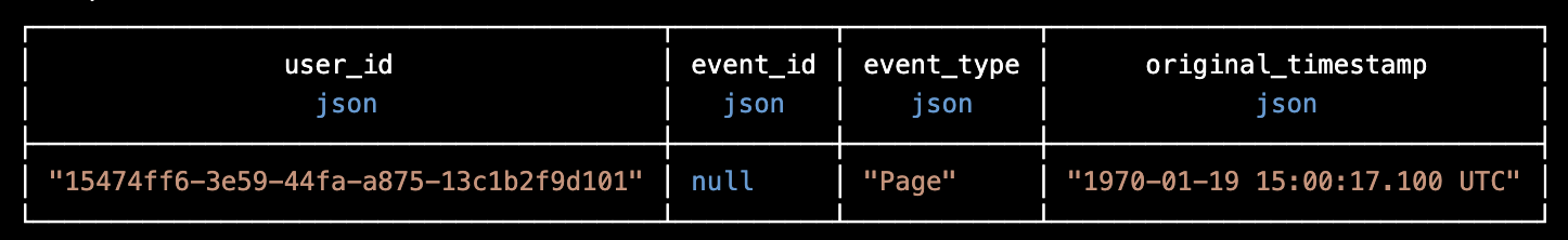
What we did was to use the json_extract function of DuckDB to extract only the fields we care about. In this case we want:

1. user_id, so we can create sessions for each user_id
2. event_type, this is not necessary but it might be helpful to have some meta around our data
3. original_timestamp, this is obviously needed as we need to perform calculations based on time to create the sessions
4. event_id, we want a way to link back to the initial record.

If you paid attention to the above results you will notice a few issues

• All the data types are of type json
• The event_id is null

The first issue is expected and it’s part of our job to take care of it as we build our code. The second issue though is weird, shouldn’t the event have a unique id? Is this a coincidence?

Let’s see what we can figure out, but first let’s make our lives a bit easier by executing the following sql

D create view extracted_json as 
		select json_extract(json, '$.context.traits.id') as user_id,
			json_extract(json, '$.message_id') as event_id, 
			json_extract(json, '$.event_type') as event_type, 
			json_extract(json, 'original_timestamp') as original_timestamp 
		from js 
		limit 1;

We create a view so we don’t have to run the long query above every time we want to query it. Now let’s see what we can learn about the message_id column.

D select distinct event_id from extracted_json;

┌──────────┐
│ event_id │
│   json   │
├──────────┤
│ null     │
└──────────┘

The above query gives us back all the distinct values of the column and for event_id everything is null which is not good!

Obviously this shouldn’t have happened, the events should have a unique ID but reality is far from ideal and issues like that can always happen, so how do we move forward with this dirty data set we have?

If we need the event_id, we have two options:

1. Check our pipelines to see why the event_id wasn’t captured. Maybe when you extracted the data the pipeline ignored the field or maybe it wasn’t even captured at the first place.
2. Come up with a solution to add a unique id for our current data set.

Although we don’t need the event_id for our sessionization example, we’ll go through an example of how this could be done. Keep in mind that there are many different ways to do it actually!

The options:

1. A common way to create unique IDs is to use hashing. This will also allow you to deduplicate your data if you need to. The way to do it is by using a hashing function, i.e. md5, and hash the whole row. In this case if two rows are completely identical, the generated hashes will be equal.
2. An even easier way to do it, is to just add the position of the row in the table as the id. This is going to ensure uniqueness of the id but it won’t help you in deduplicating the data.
3. Use something like the uuid DuckdDB function that returns random uuids and hope that random also means unique.

In our case we will opt for the second option as it’s the easier one but please feel free to to try and do the first!

Also, to perform this task is an awesome gentle introduction into window functions as we will use our first window function.

See the following SQL:

D select user_id, 
					event_type, 
					original_timestamp, 
					row_number() over () as event_idx 
from extracted_json 
limit 1;

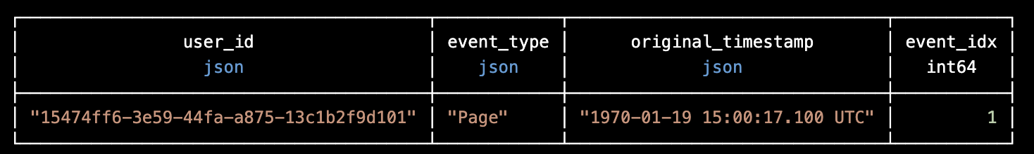
We excluded event_id as part of cleaning our dataset and used row_number() to get the row number and use it as the id for the event. See the use of the over keyword? That’s an indication that row_number() is a window function.

In our case we didn’t want to have partitions because that wouldn’t generate globally unique ids, so we run the window function over the whole table.

Now that we have a way to generate unique ids let’s figure out how to get rid of the json type and turn it into something more useful.

Consider the following SQL query:

D select cast(user_id as string) as user_id from extracted_json limit 1;

┌────────────────────────────────────────┐
│                user_id                 │
│                varchar                 │
├────────────────────────────────────────┤
│ "15474ff6-3e59-44fa-a875-13c1b2f9d101" │
└────────────────────────────────────────┘

The function CAST is what we need here. We ask DuckDB to take the JSON type and turn it into a String and in this case it worked perfectly as you can see by the result.

Now consider the following:

D select cast(original_timestamp as timestamp) as original_timestamp 
from extracted_json 
limit 1;

Error: Conversion Error: timestamp field value out of range: ""1970-01-19 15:00:17.100 UTC"", 
expected format is (YYYY-MM-DD HH:MM:SS[.US][±HH:MM| ZONE])

Ouch, we got an error! Apparently the format we used for the date cannot be converted into a timestamp. We need to fix this before we move on.

Check the following query:

SELECT 
  CASE 
    WHEN original_timestamp LIKE '%.%' THEN strptime(trim(both '"' FROM original_timestamp), '%Y-%m-%d %H:%M:%S.%f UTC') 
    ELSE strptime(trim(both '"' FROM original_timestamp), '%Y-%m-%d %H:%M:%S UTC') 
  END AS parsed_timestamp
FROM extracted_json limit 1;

┌──────────────────────────┐
│     parsed_timestamp     │
│        timestamp         │
├──────────────────────────┤
│ 1970-01-19 15:00:17.0001 │
└──────────────────────────┘

we did it! So what happens with the above query.

1. First we need to trim the character “ from both the beginning and the end of the value.
2. Then we need to account for two cases, one where milliseconds exist in time and one for when they don’t. Again this is an issue with the generation of the data and we have to fix it here.
3. For each case, we use strptime to get a timestamp out of the string.

CASE is the equivalent of IF-THEN-ELSE statements in SQL.

Now that we have figured out everything, let’s transform our raw data into something easier to work with by creating another view.

SELECT 
   CASE 
 WHEN original_timestamp LIKE '%.%' THEN strptime(trim(both '"' FROM original_timestamp), '%Y-%m-%d %H:%M:%S.%f UTC') 
     ELSE strptime(trim(both '"' FROM original_timestamp), '%Y-%m-%d %H:%M:%S UTC') 
   END AS p_timestamp,
   cast(user_id as string) as user_id,
   cast(event_type as string) as event_type,
   row_number() over () as event_id
 FROM extracted_json limit 1;

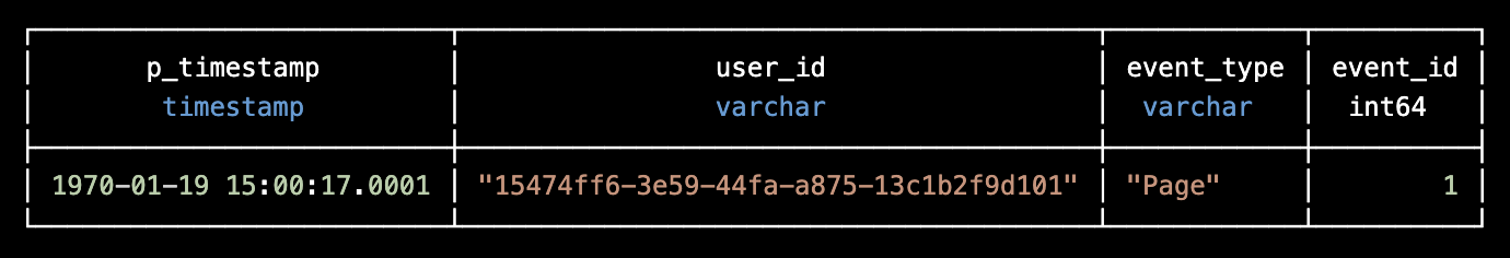
and we have what we need! Now let’s create a view so we can work with it easily.

create view events as SELECT 
   CASE 
 WHEN original_timestamp LIKE '%.%' THEN strptime(trim(both '"' FROM original_timestamp), '%Y-%m-%d %H:%M:%S.%f UTC') 
     ELSE strptime(trim(both '"' FROM original_timestamp), '%Y-%m-%d %H:%M:%S UTC') 
   END AS p_timestamp,
   cast(user_id as string) as user_id,
   cast(event_type as string) as event_type,
   row_number() over () as event_id
 FROM extracted_json;

D select count(*) from events;

┌──────────────┐
│ count_star() │
│    int64     │
├──────────────┤
│        31415 │
└──────────────┘

And

D describe events;

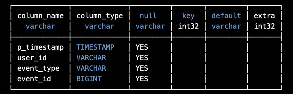We are good to go!

I know it’s been a journey so far, but we already worked with a window function and we also did something important, cleaned and prepared our data!

This is big part of the work involved with data.

Now let’s go back to sessions. Remember the definition of a session?

If you remember the examples you gave earlier you might have already figured out that LAG is probably a great candidate for helping us with our problem here, let’s see how.

consider the following query:

WITH events_enriched AS (
  SELECT 
    user_id, 
    p_timestamp, 
    LAG(p_timestamp) OVER (PARTITION BY user_id ORDER BY p_timestamp ASC) AS prev_timestamp
  FROM events
), 
sessions AS (
  SELECT 
    user_id, 
    p_timestamp, 
    prev_timestamp, 
    SUM(CASE 
      WHEN p_timestamp - prev_timestamp > interval '30 minutes' OR prev_timestamp IS NULL THEN 1 
      ELSE 0 
    END) OVER (PARTITION BY user_id ORDER BY p_timestamp ASC) AS session_id
  FROM events_enriched
)
SELECT user_id, p_timestamp, session_id
FROM sessions
ORDER BY user_id, p_timestamp ASC;

Here we are also using CTEs that we haven’t talked yet, but don’t worry that much if you find this WITH syntax new. It’s mainly a way to organize the code and make it cleaner.

As you can see we start by enriching our events by adding the previous timestamp as a new column. To do that we of course use LAG and windows! The way that part of the query works should be clear to you by now.

The second part is the session creation. Here we are creating a new column that tracks the session id. The interesting part is what’s inside the SUM clause.

Again here you see the beauty of the declarative nature of SQL. We can add a 0 or 1 based on the difference between the two columns that represent the event times.

Once again, we use SUM as a window function, remember that all aggregation functions are window functions, to calculate the session id for each user.

With that query we will end up with a result like this, I will limit the results to 10 for convenience.

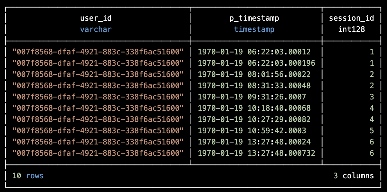
Isn’t pretty? 😊

Conclusion

Window functions are super powerful. If you master the concepts behind them you’ll be able to write some very expressive and elegant SQL code.

They might require from you to change the way you are thinking, especially if you are coming from more imperative programming languages but it won’t take that long to get comfortable with them.

I hope that the examples I gave were helpful!

In any case, please let me know of what you think and what else you’d like to see as a SQL tutorial.

References

DuckDB Intervals Documentation

DuckDB Timestamp Documentation

DuckDB Text Functions Documentation

DuckDB Date Formats Documentation

DuckDB JSON Extension Documentation

DuckDB Window Functions Documentation

DuckDB Installation Documentation

RudderStack Event Schema Spec

PostgreSQL Window Functions Documentation

Snowflake Window Functions Documentation

Fake Events Generator Source Code

Sample Event Data